The field of robotics is experiencing an algorithmic shift towards VLAs (Vision Language Action) models - teaching transformers to “speak” robot actions in the physical world.
In this post, I’ll:
- Demystify robot actions - what do VLAs output to make robots move.
- Review how action representations have evolved over the past couple of years.
I don’t have a robotics background so all of this is quite new to me, and I’ve always been perplexed by the bridging of what must happen between a model outputting tokens to an actual arm flipping a pancake. What do robot actions actually look like?
LeRobot - the gateway drug
Recently the barrier of entry to this area has dropped drastically. You don’t need to spend thousands of dollars for industrial hardware just to get started. There’s open-source 3D printable arms, pre-assembled motor kits, open cross-embodiment datasets and quite a few pre-trained foundation models you can pick up and finetune for your purposes.
The LeRobot project from Hugging Face is a great resource for getting started with fundamentals of robotics ML. There’s even cheap 3D designs and motor kits you can get that work out of the box with their software stack. So, to build intuition around driving robot actions we’ll look at the LeRobot hardware & software stack in the first part of this writeup.
For my home setup I got the Koch v1.1 which is based on dynamixel motors. After building the arms one of the first examples they have you do is teleoperation - controlling a follower arm manually using a leader arm. Teleop is a common approach for gathering training data for your ML models. Here’s the arms in action:
Looking at the code it’s surprisingly simple:
while True:
    action = teleop_device.get_action()
    robot.send_action(action)
the whole teleop example was just a Python while loop! Where are the days of programming MSP430 registers with raw C while looking up pages of datasheets on how to do PWM…
So what happens when you run robot.send_action()? Let’s take a peek under the hood.
How do things move? Motors!
A servo motor can turn a number of degrees based on the number we write to its controller board - not very fun on its own. Now screw on a piece of plastic to it and congratulations - you now have a very primitive robotic appendage.
Controlling a single motor
Let’s say you just want to control a single motor of an arm, e.g. one of the Dynamixel motors that came with the Koch v1.1 follower arm kit. We’ll use the Python API which the vendor provides.
Some of our code will depend on the specific motor model, e.g. below I’m showing you an example of moving an XL330 which is controlling the gripper of my follower arm.
from dynamixel_sdk import PortHandler, PacketHandler

protocol = 2.0 # seems to be default
device = '/dev/ttyACM1' # usb device connected to dynamixel motors
motor_id = 6 # I set this as the gripper ID
baudrate = 1_000_000 # Default in lerobot

# Addresses from
# https://emanual.robotis.com/docs/en/dxl/x/xl330-m077/#control-table
ADDR_TORQUE_ENABLE=64
ADDR_GOAL_POSITION = 116
ADDR_PRESENT_POSITION = 132

# Boilerplate communication setup
portHandler = PortHandler(device)
packetHandler = PacketHandler(protocol)
portHandler.openPort()
portHandler.setBaudRate(baudrate)

# Enable torque
packetHandler.write1ByteTxRx(portHandler, MOTOR_ID, ADDR_TORQUE_ENABLE, 1)

# Read current position of motor
current_position, _, _ = packetHandler.read4ByteTxRx(portHandler, motor_id, ADDR_PRESENT_POSITION)

# Calculate goal position by adding how much we want to rotate
goal_position = current_position + int((45/360) * 4095) # move 45 degrees

# The bit that makes the motor move
packetHandler.write4ByteTxRx(portHandler, motor_id, ADDR_GOAL_POSITION, goal_position)
Note that we need to do a little math to get the magic number to send to the controller board - each motor will typically have a fixed resolution. The Dynamixel XL330’s have 12bit encoders which means there’s 4096 possible position values you can write to them, hence we normalize by full rotation (360) and scale by our max resolution (4096, actually 4095 because Python uses 0-based indexing).
If you run this code (assuming your USB port and motor ID is setup like mine), you’ll see the gripper motor twist quickly by ~45 degrees.
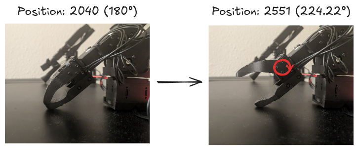
Moving the gripper of a Koch v1.1 robot arm by 45 degrees programmatically.
Do note I say quickly - these things can be fast, but in an ideal world we want our robot motions to be smooth so it doesn’t hurt anyone or itself. Of course there’s a time and place, but you do want to avoid the jittery-ness that come from big jumps between predicted motor positions.
Moving an arm (multiple motors)
Let’s scale this up a bit: each motor with an appendage adds a degree of freedom (DoF) to your robot. DoF just means how many joints the robot has, each joint being actioned by a motor. Since we’re dealing with multiple motors on a bus, now we need to make multiple API calls to different motor IDs. Luckily libraries like LeRobot already exist where all the low-level API calls are abstracted for us.
Recall the teleop Python loop from earlier:
while True:
    action = teleop_device.get_action()
    robot.send_action(action)
If you print out the action it’s just a dict where the keys are the joint names corresponding to the motors in the arm:
action = teleop_device.get_action()
print(action)
# Output:
{'shoulder_pan.pos': 4.322344322344335,
 'shoulder_lift.pos': -99.59514170040485,
 'elbow_flex.pos': -90.30362389813908,
 'wrist_flex.pos': 4.133685136323663,
 'wrist_roll.pos': 4.224664224664238,
 'gripper.pos': 49.2676431424767}
In LeRobot the joint positions (motor states) are normalized to [-100,100], these correspond to maximum possible rotations in each joint after calibration - so if it can physically only turn 45 degrees that position will correspond to 100 in our action dict, which at runtime will get converted to the proper resolution the motor firmware accepts.
# Raise wrist and fully open gripper
action['wrist_flex.pos'] = 50.0
action['gripper.pos'] = 100.0
robot.send_action(action)
So to control the robot all you need to do is edit this dict and send it to the robo arm using robot.send_action(). You just write numbers and the arm moves! Just keep in mind that these normalized joint positions need to be converted to integer values before being sent off to the controller.
Joint space vs end-effector control
Before diving into the policies and VLAs I want to cover two major control modes - this really confused me when started reading robotics papers because both are commonly used. Directly setting the motor positions like we do with LeRobot is called joint-space control.
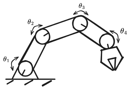
Joint control involves writing the motor positions for each joint of the robot directly.
But it’s also common to encounter actions represented with cartesian coordinates (x/y/z) and rotation parameters (roll/pitch/yaw) - in VLA literature I’ve mostly seen this called end-effector (EF) control (sometimes it’s also called task-space control e.g. MathWorks documentation).
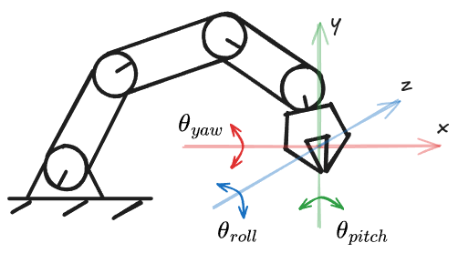
EF control tracks only the gripper position and rotation. An additional inverse kinematics (IK) stage is required to calculate the joint angles.
In EF control mode the model has to learn the position of the gripper (the end-effector) in a 3D coordinate space as well as the angles that determine the rotation of it. For a 7 DoF arm (7 joints including the gripper), both control modes will require the same number of action representations.
| Control mode | Action representation |
|---|---|
| Joint control | $\theta_{1}$, $\theta_{2}$, $\theta_{3}$, $\theta_{4}$, $\theta_{5}$, $\theta_{6}$, $\theta_{7}$ |
| EF control | $\Delta x$, $\Delta y$, $\Delta z$, $\theta_{roll}$, $\theta_{pitch}$, $\theta_{yaw}$, $\theta_{gripper}$ |
EF control has a nice advantage of being more embodiment agnostic - since it only logs the position and rotation of the effector it doesn’t really matter if the arm is 5 DoF or 8 DoF - the action space will remain 7. A separate module based on Inverse Kinematics (IK) is responsible for converting end-effector position and rotation into individual joint angles.
I liked this nice writeup on wandb.ai comparing the two control modes. EF seems like the “easier” option to learn by a model, because direct joint control requires it to implicitly learn IK. However it does seem like giving the policy direct control over the robot joints makes sense as it’s more of an end-to-end process without relying on intermediary human-crafted IK solvers.
If you look at the past efforts on robotics data aggregation, within efforts like Open-X Embodiment (O’Neill et al., 2023) most of the dataset were EF control. More recent collective - the DROID dataset (Khazatsky et al., 2024) collected both joint space and EF space trajectories. This year HuggingFace released SmolVLA (Shukor et al., 2025) trained with community sourced datasets composed primarily from joint space control data (as far as I can tell). It does seem likely that we are trending towards joint control as the dominant mode for end-to-end trained robotics policies. But maybe there’s some advantages to EF that I’m not grokking yet and we want it to stick around - guess we’ll see!
We’ve built up some intuition on what actions actually look like and how to control robots programmatically. Now how do we get robots to do this autonomously? This is where policies come in.
Robot policies
These days policies are almost analogous to machine learning (ML) models. Think of them as black boxes that take state (proprioception, observation) as an input and map it to actions which we’re very familiar with at this point. Words like proprioception might sound daunting at first but typically it’s just the readout of the joint positions on your robot.
Figuring out the numbers that determine the joint angles is what we train our policy to do. Here’s a simplified flow for a 4 DoF arm being controlled by a robotics policy:
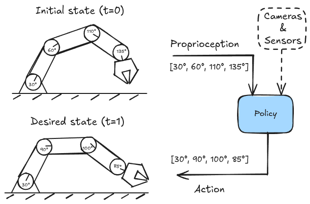
High level overview of a robot arm policy. It takes proprioception (joint angles) as input and outputs new joint angles based on observation data.
Instead of us manually typing in numbers to move the joints of the arm, they get generated autonomously by this policy.
Imitation learning vs generalists
Note that in my illustration above there’s no such thing as a directive. This policy only sees camera feed, joint positions and maybe some sensor readings. How does it know what its task is?
Imitation learning
A lot of prior work on policies is based on imitation learning (I’ve seen it referred to as action cloning as well). Meaning the robot can only perform one or a limited number of tasks. Think of AlphaGo - it’s brilliant at playing Go, but you can’t ask it questions or have it randomly pick up and play Yu-Gi-Oh.
In practice, imitation learning is me teleoperating a robot arm tossing clutter off my desk into a bin and recording each episode (video and joint positions). With enough episodes I could train a policy that would eventually clean the desk for me. Of course this comes with a plethora of challenges - grasping is hard because objects have different textures and weights, it’s difficult to generalize to new items, if I buy a new lamp the policy might freak out because now we’re out of distribution, etc.
I gave a toy example, but imitation learning is definitely already being deployed out there (e.g. Amazon warehouses). I also came across this fun example from Stanford Lab for Cell and Gene Medicine where they use imitation learning to mimic the way scientists shake flasks in a particular way. Getting it right just for 1 repetitive task can be deceitfully challenging!
Generalist policies
The holy grail of robotics is a generalist model that can perform a variety of different challenging tasks, but also adapt to new ones. In part, this is why humanoids are so popular right now - our world is built for the human form factor - a generalist policy running on this embodiment would be a gamechanger in various industries. Suddenly entire factories, warehouses, construction sites or even kitchens and households can be operated by autonomous robots.
I’ll leave the rant about possible dystopia/utopia scenarios for a later time - for now let’s agree there’s a big demand for the generalist and a lot of the research is building up to towards this end boss of AI.
LLMs today are as close to that as we’ve ever gotten. And if they’re not generalists right now, they sure are good at faking it. Slowly all the LLM-related innovations are making their way into embodied AI. And Vision Language Models (VLMs) are their first contact with physical world.
VLM - first foray into the physical world
Vision Language Models (VLMs) are multimodal LLMs that have been trained on both image & text data. While they don’t “speak” actions yet, they understand scenes in images. You can feed it pictures and it will be able to describe what’s in the image: what kind and how many items, or even predict how some actions might affect the scene (e.g. if the glass spilt the table would become wet). VLMs can be repurposed for a variety of downstream tasks, including robotics.
The visual processing is usually done via a vision encoder that will convert an input image into tokens of the same dimensionality as the base transformer model (LLM) alongside the text tokens.
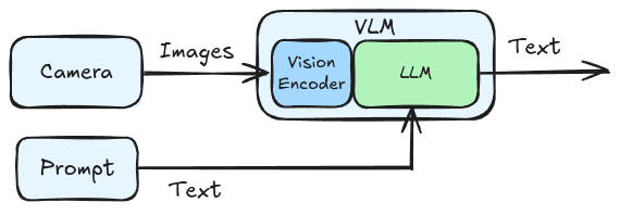
High level Vision Language Model (VLM) representation.
Present day VLMs have become the backbone of training VLAs because the prebaked image understanding is very useful. However there’s been recent studies (Chow et al., 2025) showing that their physical world understanding is still to be desired; 3D perception and world modeling are still big problems to solve, especially in the context of robotics. However it’s our first foray into the physical world using LLMs.
VLA - promising generalists
The exciting thing about VLAs is that most of them are trained to be generalists - meaning they can understand language instructions and perform multiple tasks or even long horizon tasks that need to be broken down into subgoals. In recent research they even generalize to unseen tasks in the training dataset.
VLAs add an additional modality to VLMs - they output the magic numbers we write to the motor controller APIs in the correct sequence to gracefully fold our button-up shirts.
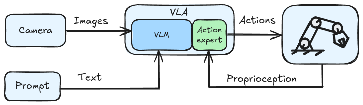
High level Vision Language Action model (VLA) representation.
Most common design pattern (but not the only one!) we’re seeing is a finetuned VLM with an additional neural network attached which specializes in the action tokens e.g. recent policies like GR00T-N1 (Bjork et al., 2025) and SmolVLA (Shukor et al., 2025) use this structure. The next section will go into much more detail of what these action tokens look like.
Evolution of action learning
Here’s a timeline of some of the more popular works in the past 2 years that I think are representative of the VLA evolution:
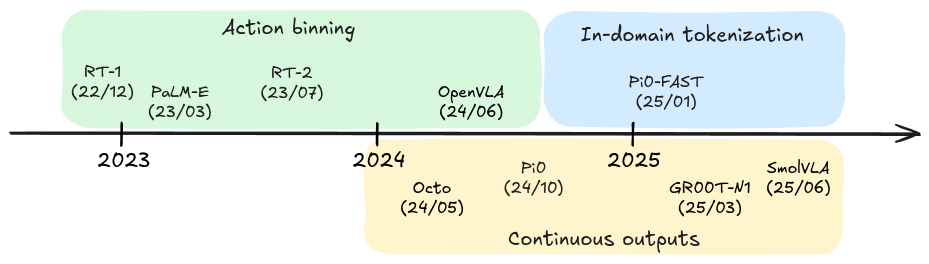
Recent VLA development timeline. We see a clear transition from action binning to diffusion-type policies.
There’s definitely more models that I haven’t included or am not even aware, but the purpose here is to understand the trends in action learning - to that end I think these have been some of the more impactful in the field.
We’ve seen a clear shift from action binning / autoregressive prediction towards action chunk inference with iterative denoising like diffusion. We also started seeing new tokenizers specifically for the robotics domain.
I’ll cover 5 examples as we walk through the timeline:
- RT-1: multimodal transformer policies emerged.
- PaLM-E: we started seeing generalist behavior from large VLMs creating plans in the physical world.
- RT-2: the first VLA - instead of using a separate policies for planning & control, now we train the LLM directly on discretized action tokens.
- Octo/Pi0: turns out diffusion-based policies work really well for generating chunks of actions, enabling operation at higher frequencies and performing more dexterous tasks.
- Pi0-FAST: we are starting to see domain-specific tokenization.
Funnily enough Google is responsible for the first 3 - always early to the party. Now let’s walk through each one to build intuition.
RT-1: robotics transformer
RT-1 (Robot Transformer) (Brohan et al., 2022) is an incredibly tiny model at 35M parameters and it operates at 3Hz, which by today’s standards is pretty slow. This network was trained from scratch (barring some CNN imagenet pretraining) on an internal dataset of 130k demonstrations collected at Google. There was no web-scale image/text pretraining, only robot demonstrations fitting the tiny model.
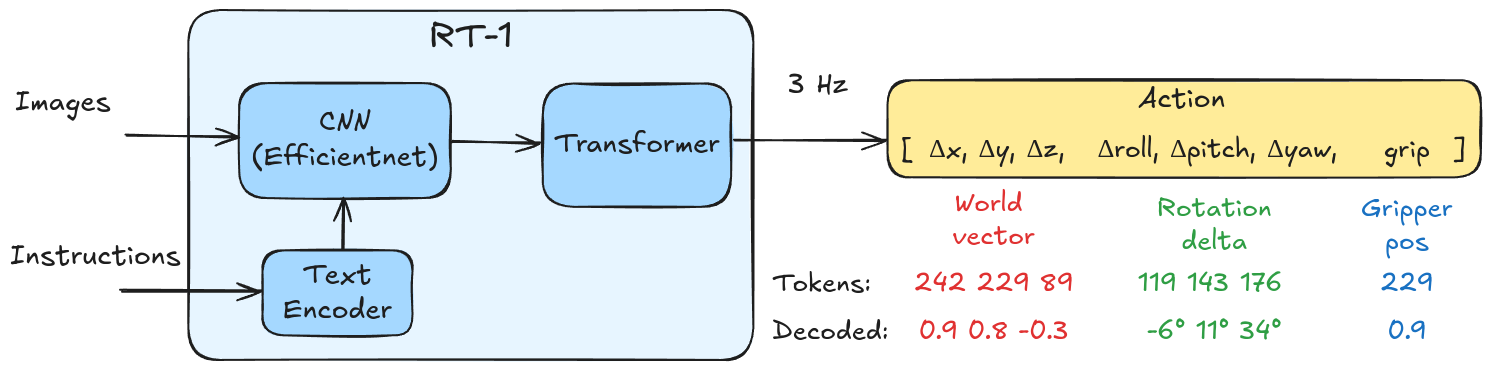
Overview of the RT-1 architecture focusing on the action tokenization scoped down to the arm control. The transformer outputs a sequence of 7 tokens which need to be de-tokenized into actions.
The architecture is composed of a CNN conditioned on text tokens, a token learner that downsamples the vision-language tokens for efficiency and a decoder-only transformer. The decoder outputs action tokens that get mapped to an end-effector control sequence for the arm and a base platform.
Action space
RT-1 utilizes action binning, where each dimension is discretized into 256 bins and the reverse is performed to get the floating point values for the controller. In the original paper the control includes a base platform as well as an arm:
- Seven for arm (x, y, z, roll, pitch, yaw, opening of the gripper)
- Three for base (x, y, yaw)
- 1 discrete variable for terminating ep (signals when the job is done and robot should stop moving)
To keep things simple we’ll ignore the platform and terminating ep, and focus solely on the arm. Note that RT-1 uses end-effector control, meaning the policy needs to output relative displacements in the cartesian coordinate space and a rotation vector of the gripper.
Action binning
So how does the binning process work? We need to convert floating point values of displacements and rotations into tokens with vocab size of 256. We can see the exact flow by looking at the tokenizer code from the open-sourced repo:
    a = tf.clip_by_value(a, spec.minimum, spec.maximum)
    # Normalize the action [batch, actions_size]
    token = (a - spec.minimum) / (spec.maximum - spec.minimum)
    # Bucket and discretize the action to vocab_size, [batch, actions_size]
    token = tf.cast(token * (self._vocab_size - 1), tf.int32)
Let’s walk through a numerical example. Start with one value from the world vector (or normalized cartesian space displacement) $\Delta{x}$.
Tokenization 0.9 (relative displacement) -> 242 (token)
1. Normalize to [0,1]: (0.9 - (-1.0)) / (1.0 - (-1.0)) = 0.95
2. Scale to vocab: 0.95 * 255 = 242.25
3. Discretize: int(242.25) = 242

Detokenization: 242 -> 0.9
1. Rescale to [0,1]: 242 / 255 = 0.949
2. Reconstruct: (0.949 * 2.0) + (-1.0) = 0.898
We got the action bounds [-1,1] from the test code of the robotics_transformer repo. Similarly, for the rotation delta we’d use the exact same steps, but the bounds would be [$-\pi/2$, $\pi/2$].
Note that in reconstruction we lose a bit of precision due to the implicit quantization that happens - 256 bins (or 8 bits of precision) provides way less resolution than modern servos are capable of. This can have a compounding effect given more DoF and, as you can imagine, might not work very well for precise granular tasks like threading a needle or picking up something small like a screw.
This model was also weak in reasoning - trained only on Google’s internal robotics dataset it didn’t have an understanding of the wider world. RT-1 was limited to simple tasks, and couldn’t execute long action horizon planning.
PaLM-E: planning
To bridge the gap between LLMs and physical embodiments the folks at Google developed PaLM-E (Pathways Language Model - Embodied) (Driess et al., 2023), a massive 562B param Vision-Language model that was trained on both web-scale data but also grounded with sensor inputs and robotics-specific inputs. This work is based on their original PaLM 540B model (Chowdhery et al., 2022). PaLM-E is a combination of the 540B PaLM and 22B ViT for image encoding.
PaLM-E doesn’t directly output action tokens. However, it is capable of chain-of-thought planning and reasoning about images. Since it can’t control a robot directly PaLM-E needs to be supplemented by an additional smaller policy that would translate low-level english instructions to motor commands.
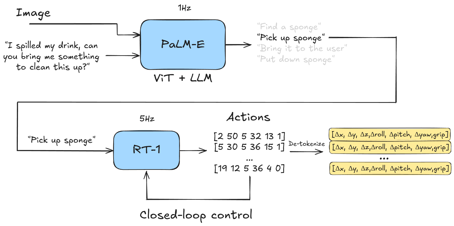
Overview of PaLM-E setup as the planner policy with RT-1 executing low-level instructions. PaLM-E breaks the task down into sub-commands, sends them to RT-1 and once RT-1 is finished it gets fed the next command.
From the PaLM-E paper it wasn’t entirely clear to me how the smaller policy works, but in Section 6.4 they mention RT-1 - so we can assume they’re RT-1 derived controllers with similar action binning.
At the time there were other related papers like SayCan (Ahn et al., 2022) that also utilized PaLM and had it select low level skills which would get passed to a smaller policy.
We are starting to see a trend towards more generalist policies that actually understand the environment and can execute longer horizon tasks. The models used were huge though, and the inference time is incredibly slow (1-5Hz). Note that Google has been running all of these models on a TPU cloud next to the robot, so nothing is embedded yet either (can you imagine a 562B param policy on an embedded device?).
RT-2: the first VLA
I believe Google coined the term VLA when presenting RT-2 (Brohan et al., 2023). It is widely regarded as the first VLA since this was the first time we saw the transfer learning of webscale data from a pre-trained VLM take place to a robotics policy.
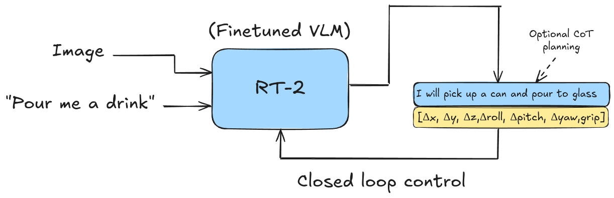
High level overview of RT-2. It's a large finetuned VLM trained to output actions directly.
The RT-2 model has 2 variants: RT-2-PaLI-X and RT-2-PaLM-E. PaLM-E we’re already familiar with, PaLI-X (Chen et al., 2023) is a similar large VLM from Google Research. Mostly cited RT-2 models are the PaLI-X variants at 55B params and a smaller one at 5B. The small model could run at ~5Hz, whereas the bigger one was reported to run at ~1-3Hz. At least in terms of speed, not much improvement over RT-1.
Action space
RT-2 uses the same action binning as RT-1, however it’s a bit more interesting at the transformer level because actions are now predicted by a finetuned VLM. This means that the vocabulary is shared, but you can’t expand the vocabulary size without changing the topology of the model architecture. The approach with RT-2 was, depending on the base VLM, to re-use existing tokens for actions.
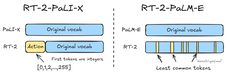
Left: the first 256 tokens of the PaLI-X vocabulary are re-used as action tokens. Right: the least used 256 tokens by PaLM-E are re-purposed as action tokens.
PaLI-X and PaLM-E had slightly different vocabularies. PaLI-X conveniently already has its first 1000 tokens dedicated to representing integers, so they reused the first 256 integers for action tokens - easy! PaLM-E didn’t have such convenient mapping, so they overwrote the 256 least used tokens - apparently this is a form of symbol tuning. OpenVLA (Kim et al., 2024) also used the same tuning method as RT-2-PaLM-E with action binning and they open-sourced their work if you want to dive a bit deeper.
Another cool implementation detail about RT-2 is that during inference they constrained the output to action token sampling only. This prevents the model from accidentally outputting “cow” when it should’ve moved the shoulder joint 8 degrees to the right.
We finally have a policy that is end-to-end trainable and can reason based on web-scale data pretraining. It can execute long horizon tasks. What are we still missing? Well…
- It’s still slow - runs at 5Hz at best.
- We’re losing precision due to action binning.
- Inference happens autoregressively and only 1 action vector is being output per observation.
People started turning to other topologies - like diffusion!
Diffusion-based VLAs: continuous output action space
The foundational diffusion policy paper (Chi et al., 2023) demonstrated that the denoising diffusion process worked surprisingly well for robot control. The policy dealt nicely with multimodality by committing to a single trajectory without jitter. Instead of outputting actions one-by-one in an autoregressive manner it would output sequences of actions in one inference attempt. Another term for this is action chunking coined in the Action Chunking Transformer paper (Zhao et al., 2023). These policies were mostly used for imitation learning - they weren’t generalist conditioned on text instructions yet, but they laid some really important groundwork for how VLAs operate today.
Octo (Ghosh et al., 2024) introduced diffusion as the robot transformer combined with a text and vision encoders, making it one of if not the first VLA with diffusion used for action token prediction. Since then diffusion has become SoTA for robot action inference: Pi0 (Black et al., 2024), GR00T-N1 (Bjork et al., 2025), SmolVLA (Shukor et al., 2025) and many others use diffusion transformers as their action experts.
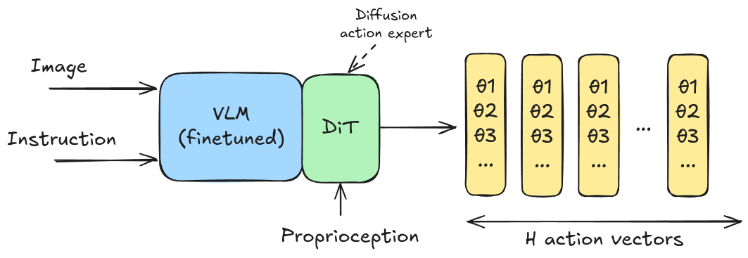
VLA composed of a VLM and diffusion transformer (DiT) as the action expert, typically connected via cross-attention. Single inference outputs H action vectors (action horizon).
Modern policies still use VLMs that are web-scale data pretrained. Similarly to Mixture of Experts (MoE) models, this VLA topology uses the VLM as the text-image expert and only routes those types of tokens through the transformer. Whereas the DiT is the action expert that deals with tokens related to actions i.e. proprioception.
Recall that previous policies we’ve seen could muster at most 5Hz. Physical Intelligence showed that their model Pi0 could perform tasks at up to 50Hz (Black et al., 2024) - that’s 10x from RT-2 days! Remember - speed here is not how many inferences we can do in a second, but how many actions per second get run.
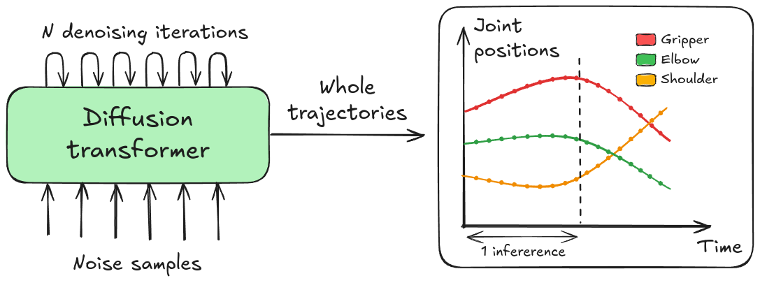
DiT action experts output entire trajectories in a single inference.
The diffusion process might need 10 denoising iterations, but this will still be a relatively low number regardless if your action horizon is 50 or 200. Comparatively auto-regressive policies will need that many transformer steps per action dimension. We also don’t need to discretize our actions anymore (action binning of RT-1/RT-2) because the diffusion process produces smooth continuous action values.
Even super recent works like from Boston Dynamics are still using diffusion for action prediction. So I don’t think it’s going away any time soon.
Of course robotics hasn’t been solved yet - so what are we still missing? Well there’s still a couple outstanding issues with SoTA VLAs, that are being worked on as we speak:
- During training VLMs tend to forget a level of world knowledge and the models lose generalizability. RT-2 was co-trained with action and original web data with action tokens in the same vocabulary as text-image tokens. This approach would be ideal to preserve generalizability, but few companies have the data and compute to replicate what Google does.
- Long horizon predictions (100+ actions) don’t guarantee most up-to-date observation data per action. E.g. once you reach the 50th action token the environment may have drastically changed because you’re running on assumptions made half a second ago.
The last action learning methodology doesn’t exactly address these issues but personally I find it really cool so I wanted to cover it as well - in-domain tokenization.
Pi0-FAST: first domain-specific tokenizer
The Frequency-space Action Sequence Tokenization (FAST) tokenizer (Pertsch et al., 2025) from Physical Intelligence was the first time I’ve seen in-domain tokenization for robotics. To me this makes so much sense, especially following what’s being going on in the LLM space. We never do character or word-level prediction anymore, today’s tokens are these information-dense representations that already come packed with information to make it easier for the transformer to make predictions. That’s basically what FAST is doing.
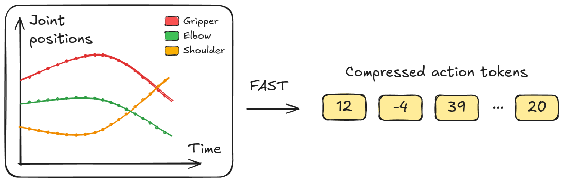
In a nutshell FAST compresses trajectories into discrete tokens. And because they're compressed the transformer model needs fewer inference steps.
There’s definitely redundancy in robotics trajectories - for example how much does the shoulder move if you’re only doing vertical arm movement with the elbow? It doesn’t. We could just compress all those 0’s into a single token.
This sparsity is exploited when you convert the time-series trajectories into the frequency domain. Typically recorded trajectories contain mostly low-frequency components, with high frequencies contributing very little to the signal, which means we can throw them away while preserving the majority of the action information. The original paper figure illustrates this nicely:
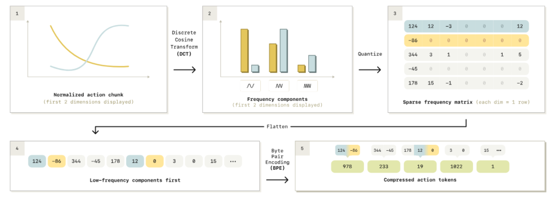
Detailed overview of the FAST algorithm.
Props to Physical Intelligence for open sourcing the tokenizer, so we can easily play around with it. Here I create some synthetic trajectories and see how good of a job it did at reconstructing the actions.
import numpy as np
from transformers import AutoProcessor

# Load tokenizer and generate sinusoidal trajectories
tokenizer = AutoProcessor.from_pretrained("physical-intelligence/fast", trust_remote_code=True)
t = np.linspace(0, 2*np.pi, 50)
trajectory = np.zeros((50, 3))

for i in range(3):
   f1, f2 = np.random.uniform([0.5, 0.2], [2.0, 1.5])
   a1, a2 = np.random.uniform([0.3, 0.2], [1.0, 0.8])
   p1, p2, offset = np.random.uniform([0, 0, -0.5], [2*np.pi, 2*np.pi, 0.5])
   trajectory[:, i] = offset + a1*np.sin(f1*t + p1) + a2*np.sin(f2*t + p2)

action_data = trajectory[None, :]  # Add batch dimension

# Tokenize and decode
tokens = tokenizer(action_data)
decoded_actions = tokenizer.decode(tokens)

print(f"Actions: {action_data.shape}, Tokens: {np.size(tokens)}, Decoded: {decoded_actions.shape}")

# Output:
Actions: (1, 50, 3), Tokens: 19, Decoded: (1, 50, 3)
Look at that! So our sequence of 50 actions (total 150 elements) got compressed to only 19 tokens, that’s 38% of the original sequence length. But recall that DCT isn’t lossless compression, so let’s take a look at the reconstructed trajectories:
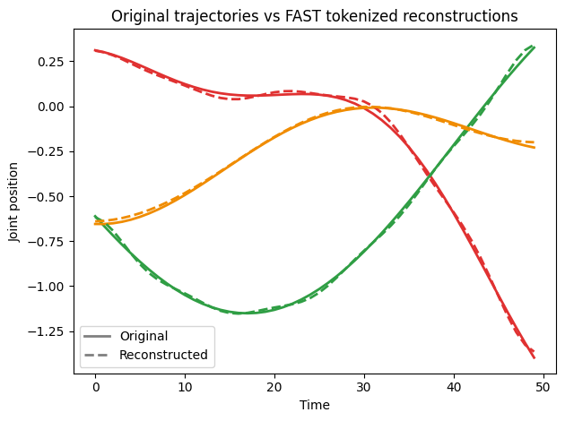
Plotting original actions vs reconstructed actions from FAST tokens. The reconstructed trajectories are a very close match to the original.
Training gets significantly simpler because the action sequence lengths become shorter. According to the paper the autoregressive pi0 model converges 5x faster with FAST. However, this is only in training. Even with FAST the autoregressive policy is still slower when computing 1 second worth of actions taking 750ms per inference compared to diffusion which takes 100ms to produce the same output.
What’s next?
In terms of action representation strategy I think these flow matching, diffusion-style heads will stay with us for a while. Though I can’t believe I haven’t seen more work on tokenization. There’s a lot of scope for compressing actions efficiently, lots of signal processing techniques waiting to be re-discovered. That said, there are plenty of other pressing issues to solve.
Right now we still don’t have true generalists walking around in our houses learning tasks on the go. We still need that AGI. One problem with training VLAs today is that the backprop gradients from the action expert overwrite VLM weights - making the model dumber. There’s been a lot of pretty cool developments to overcome some of these issues. E.g. Physical Intelligence (Driess et al., 2025) introduced the concept of Knowledge Insulation (KI) to preserve the VLMs integrity.
Latency and speed are also big issues. Predicting action chunks introduces big pauses between inference and action, and like I mentioned before you can’t operate on too long of an action horizon because you’re acting on outdated observation info. Recently Physical Intelligence released a paper on real-time action chunking, where they execute the actions and asynchronously start predicting the next chunk (Black et al., 2025). HuggingFace implemented a similar asynchronous runtime for SmolVLA and reported 2x the throughput with this approach.
Accuracy and generalizability will come as models improve - currently robotics policies are following VLMs and these things are only getting smarter. What’s even more exciting is that the small open-source models are becoming more capable! Smaller models - more accessible to community - I’m a big fan of the new Gemma models that got released with official quantized checkpoints, I hope this becomes more of a trend and we’ll start seeing VLAs built on top of these soon enough.
Closing
Hopefully this writeup clarified what the “A” in VLA is. It’s really impressive how much was achieved in just a couple years.
I don’t know how close we really are to true generalists - honestly, it might not happen until AGI arrives. But if you want to get in on the action then right now is the best time to dive into robotics.
Even without hardware you can make significant contributions just on the software side: finetune Pi0 in sim or play around with signal processing techniques to come up with more efficient tokenizers!
TTFN